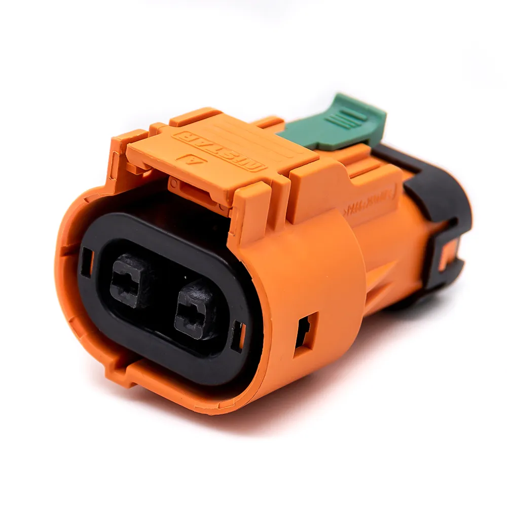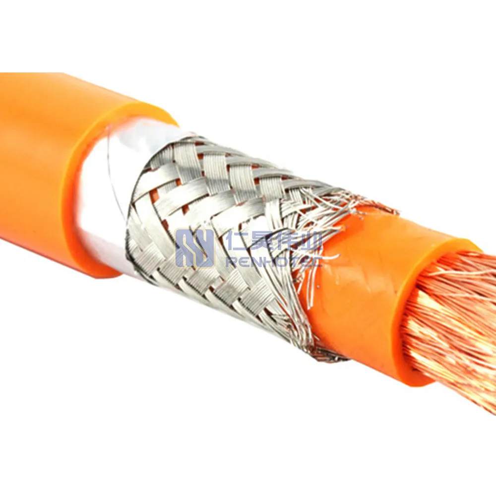
60A - 120A
125A - 200A
250A - 350A
400A - 480A
On this page
Engineering guide
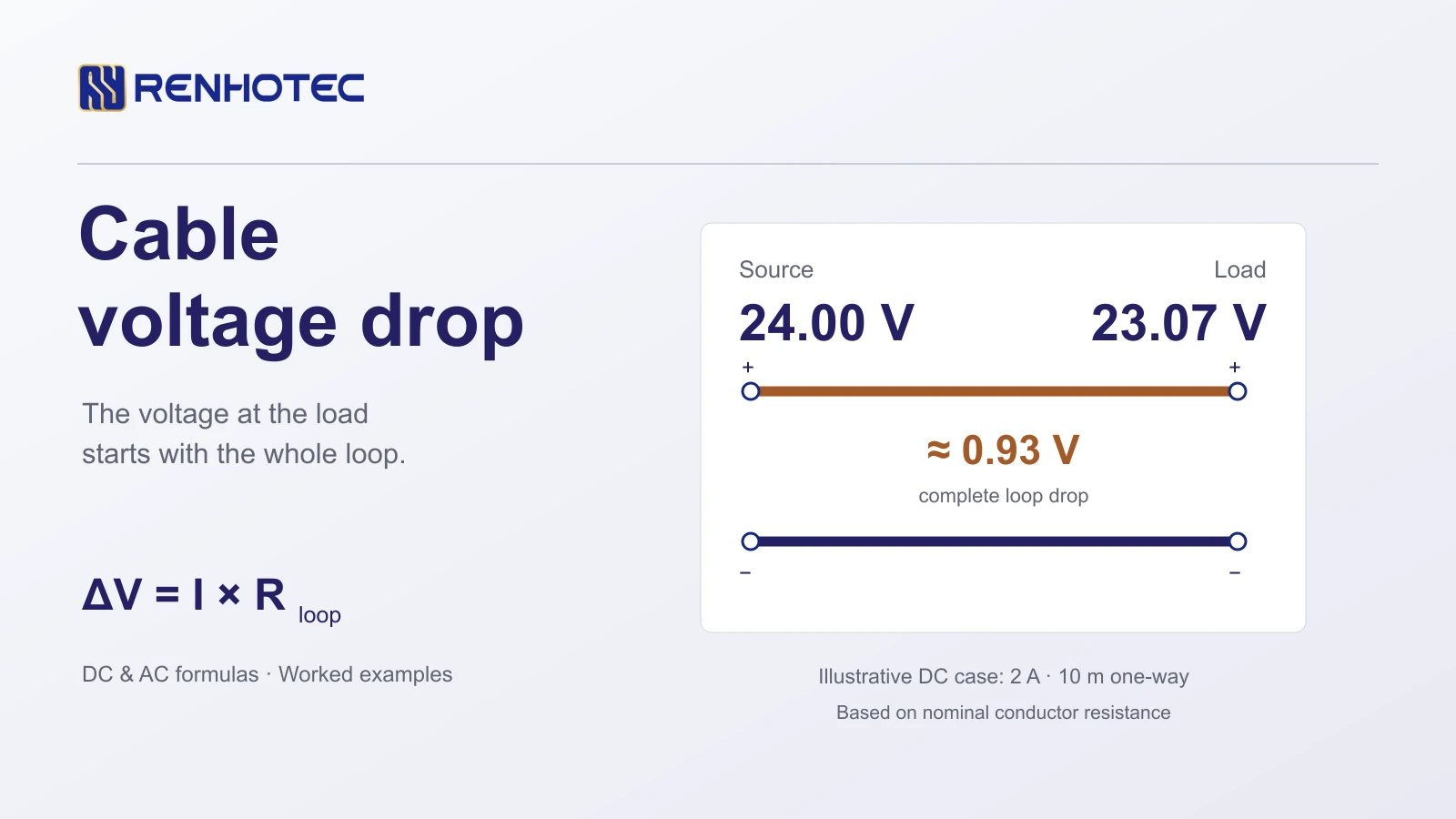
When current flows through a cable between a power source and a load, the resistance—and in AC circuits, inductive reactance—of the conductors produces a voltage drop along the path. In a DC circuit, voltage drop follows : for a two-wire run built with two identical conductors of one-way length and single-conductor resistance per meter , current travels meters to the load and meters back, making the total loop resistance .
For steady-state AC circuits, the calculation must match the supply configuration ( for single-phase or for balanced three-phase line-to-line) and account for conductor resistance , reactance , and load power factor (). Whether the resulting load-end voltage is acceptable depends on the voltage budget between your chosen reference terminals—comparing the estimated terminal voltage against the equipment's minimum allowable input voltage after accounting for series connector, fuse, and switch losses.
Selecting the right equation starts with verifying how cable length and resistance are defined in your specifications. Mixing up one-way routing distance with round-trip conductor path length, or multiplying a pre-tabulated circuit factor a second time, will skew the result.
When you specify a two-conductor cable assembly, is the one-way physical distance () from the source to the load. Electrically, current must flow out through the supply conductor and return through the return conductor to complete the circuit, as explained in the Victron Energy Wiring Unlimited guide.
For a two-wire circuit using two identical conductors of one-way length (in ) and single-conductor resistance (in ), the complete conductor loop resistance is:
If the positive and negative conductors follow routes of different lengths or use different wire cross-sections, calculate the resistance of each wire leg separately and sum them:
Check whether the stated value in your reference document is single-conductor resistance or loop resistance before multiplying by . Cable datasheets typically list resistance per individual core (, , or ), which requires multiplying by for an equal-leg two-wire loop. If a table already specifies loop resistance for a pair, use that value directly.
Along an assembled circuit, bulk wire is not the only series resistance. Crimp terminations, mated connector contacts, fuses, and switches add voltage loss along the path:
In low-voltage circuits with tight margins, include connector contact resistance and protection elements in the path budget alongside the conductors. For how contact resistance is evaluated separately from bulk wire resistance, see Connector Resistance & Hipot Tests.
In the DC equation below, is current in amperes (), is one-way cable length in meters (), and is single-conductor resistance in ohms per meter ():
The final form applies to two equal conductors.
In the steady-state AC equations below—following the conventions in the Schneider Electric Electrical Installation Guide— is line current in amperes (), is one-way cable length in kilometers (), and and are single-conductor AC resistance and inductive reactance in ohms per kilometer () at the applicable operating conditions. These expressions apply to approximate sinusoidal steady-state conditions with a lagging (inductive) power factor , where is the phase angle between voltage and current and (leading capacitive loads cannot simply use , and unbalanced three-phase or non-sinusoidal currents require matching circuit models):
When applying the AC equations, keep three rules in mind:
If a load (such as a regulated DC-DC converter or switch-mode power supply) maintains approximately constant electrical input power at its input terminals within its regulated operating range, a drop in terminal voltage increases its input current draw according to . Here is the electrical input power at the load terminals (including converter efficiency, not the downstream output power alone). When voltage drop is significant, check the device's input current specification at the reduced terminal voltage rather than relying on .
Manufacturer catalogs and installation guides often publish a voltage drop coefficient for a given cable construction, installation method, operating temperature, circuit type, and power factor. Because already embeds the or circuit multiplier and the impedance term, you simply multiply , current, and one-way length—without multiplying by or again.
With current in amperes and the result in volts, match the length unit to the unit of :
Although equals numerically, is a voltage drop factor for those specified conditions (not a loop resistance), and the conversion is required when length is entered in meters.
Translating a cable datasheet entry into or requires checking the unit, tolerance type, reference temperature, and conductor row before starting the calculation.
Because , convert single-conductor resistance from to ohms per meter () by dividing by :
In metric specifications, resistance is typically listed in or milliohms per meter (). Because and , these two units are numerically identical:
| Datasheet Unit | To Get | To Get (or ) |
|---|---|---|
| Divide by | Divide by | |
| Divide by | Same numerical value () | |
| Divide by | Same numerical value () |
Check three specification details alongside the DCR number:
Nom.) vs. Maximum (Max.) DCR: Control and instrumentation cable datasheets often publish a nominal DCR rather than a guaranteed maximum. Nominal DCR provides a baseline estimate, whereas worst-case margin verification requires checking maximum DCR limits. For how nominal and maximum parameters are presented on component datasheets, see How to Read a Connector Datasheet.Shielded cables list electrical parameters for both the insulated cores and the shield. On the Belden 8760 Technical Data Sheet, Conductor DCR appears right above Nom. Outer Shield DCR. In a two-conductor shielded control cable like Belden 8760, the two insulated copper cores carry the circuit current while the foil shield and drain wire provide electromagnetic screening. Use Conductor DCR when calculating the supply-and-return loop resistance. For shield grounding and EMC practices, see the Cable Shielding Guide.
The two examples below demonstrate the calculation flow for a control cable run and a balanced three-phase AC motor feeder. Unrounded intermediate values are retained inside the calculations and rounded for display.
The Belden 8760 Technical Data Sheet (Rev 0.667, dated 2026-02-20; product page) supplies the cable data. The operating values below are assumed for this calculation, with both insulated cores used as equal-length supply and return legs.
Cable datasheet · Belden 8760
7.06 Ω/1000 ft
Nominal conductor DCR
One pair · 18 AWG · 16 × 30 AWG tinned copper
Reference temperature is not stated in the DCR field.
Assumed operating values
Because voltage drop scales linearly with length at constant current, halving the one-way run to halves the conductor drop to . To complete the circuit verification, check the load's minimum required input voltage () and account for series connector/fuse drops, supply output tolerance, and operating temperature rise.
This published example from the Schneider Electric Electrical Installation Guide (Fig. G30 / Example 1) evaluates a balanced three-phase motor fed through a copper cable with a one-way length of , using () from the guide's copper, balanced-three-phase columns. The running and starting coefficients correspond to the power factors shown below:
| Parameter | Running | Starting |
|---|---|---|
| Line current () | ||
| Power factor () | ||
| Tabulated factor () |
Running:
Starting:
The upstream network also loses voltage. In Schneider's example, its running drop is at a total distribution-board current of . During starting, the assumed upstream current is ; the guide scales the upstream drop proportionally to . The chart separates this upstream contribution from the feeder loss.
Even though starting current is the running current ( vs. ), the drop in power factor from to changes from to , yielding a feeder drop rather than . Running and starting conditions must therefore be calculated separately using their respective current and power factor, and compared against the equipment manufacturer's allowable input/starting voltage limits and the governing installation standard.
Once you can calculate voltage drop for a given cable, the same relationships let you establish an allowable voltage budget, back-calculate maximum cable length or minimum conductor cross-section, and verify performance under load.
Commonly cited limits such as (lighting) and (other uses)—as summarized in the Schneider Electric guide to IEC 60364-5-52 Table G.52.1—apply to installations supplied directly from a public low-voltage distribution system under normal steady-state operation, with variations across national standards.
For a dedicated two-wire DC circuit, determine the allowable conductor voltage drop () directly from the voltage limits at your chosen reference terminals:
At nonzero current, if , no positive cable length can satisfy the budget without raising the minimum source voltage, reducing series component losses, or selecting equipment with a wider input range. If is unknown, report the estimated drop and load voltage as outputs without assigning a pass/fail result.
With a positive conductor budget for an equal-leg two-wire DC run, rearrange to solve for the maximum one-way length:
Using the current and Belden 8760 nominal resistance () from the DC example with an assumed conductor-only budget of gives:
Because this figure is an estimate based on an assumed conductor budget and nominal DCR, verify final run length against maximum DCR limits and operating temperature.
When the one-way distance is fixed on an equal-leg two-wire DC circuit made of a single conductor material, you can screen for a candidate conductor cross-sectional area using consistent units:
Use in meters, in amperes, and in volts to obtain in .
Here is the conductor material's resistivity (in ) at an explicitly stated material specification and operating temperature. After computing , select a standard conductor size whose cross-sectional area is at least (see the AWG to mm² Wire Size Chart to match metric area to AWG sizes), then pull that specific cable's datasheet DCR at the operating temperature to recalculate . For single-phase or three-phase AC feeders, verify the candidate cable using the AC equations and its corresponding and (or ) values from the first section.
Meeting satisfies the voltage-drop criterion only. Final cable selection must also verify three independent requirements:
When specifying custom assemblies on engineering drawings, stating the one-way length, operating current, and maximum allowable loop resistance alongside connector part numbers keeps electrical and mechanical tolerances aligned—see Cable Assembly vs. Wire Harness.
When checking an installed low-voltage DC circuit with a multimeter, a voltage reading with the load idle or disconnected can miss excessive path resistance. For the same resistance, lower current produces less loss: a reading close to source voltage at light load does not establish the voltage available at full load.
The troubleshooting procedure in the Victron SmartSolar MPPT 100/30 & 100/50 manual (§8.6.3) illustrates how to check low-voltage DC cabling under load:
The voltage difference between those two terminal pairs reflects the total voltage loss along the entire path between the probes, including both conductors and any inline fuses, switches, or terminal joints. Compare that difference with the allowable path budget at the measured current. These readings give the combined loss; locating a suspect termination requires separate checks of individual sections.